PLOUTOS MANUAL
Table of contents
I. Introduction
II. Select reaction data
III. Plotter
IV. Solver
V. Default cases
I. Introduction
PLOUTOS is a visualization and manipulation toolkit for EIRENE A&M databases AMJUEL, HYDHEL and H2VIBR (see Documentation). It is distributed under EIRENE license and it is available here (to get access click Ploutos on the left column - restricted to registered users).
II. Select reaction data
Reactions data in AMJUEL, HYDHEL and H2VIBR databases refers to those processes with a background projectile (electron or bulk ion) impacting on a target (atom, molecule, test or bulk ion). EIRENE needs reaction rates and in some cases also cross sections (charge-exchange collissions) and interaction potentials (elastic collisions).
PLOUTOS initial page contains the following 4 tables of reaction data
- collisions with e, where e stands for electrons,
- collisions with p, where p stands for protons,
- collisions with H, meaning collisions with hydrogenic A&M species,
- collisions with He, meaning collisions with helium species.
Each table is organized such that the reaction data for the same physical process are grouped together and shown as consecutive rows. The following column features are present:
- number: a label for the physical process in the form of three integer digits split by dots, for instance 2.1.5 for hydrogen ionization by electron impact (Janev notation),
- reaction: the formula of the reaction, which uniquely identifies the group of reactions corresponding to the same physical process and different data in the same goup may refer to different models and/or different particle internal states (electronic, vibrational and/or rotational ones).
- range: the limits of validity of the data in energy for cross sections (section H.1), in temperature for those rates in sections H.2 and H.8, in temperature and energy for those rates in sections H.3 and H.9, in temperature and density for those rates in sections H.4 and H.10.
- reference: the main reference from which data are taken,
- data type: the type of data, whether they are experimental or calculated from a theory,
- peculiar properties: a general comment about the data, as for instance the theoretical model used for computation, some specific properties or features,
- generation: a label to keep track of the insertion of new data: 0 for all reaction at present, it will increase in next developments,
- data origin: a specification of how the data have been obtained, for instance whether it is the original fit present in the reference, or it is an improved fit or for experimental data whether it is the fit of the original data,
- File/chapter: the corresponding chapter (see next table for the quantity in each chapter) and database (AMJUEL, HYDHEL or H2VIBR).
| Chapter |
Quantity |
Variables |
Comments |
| H.0 |
interaction potentials |
energy |
for elastic processes |
| H.1 |
cross section |
energy |
laboratory frame (comoving with the target species) |
| H.2 |
reaction rate |
temperature |
vanishing target energy and non-drifting background Maxwellian distribution |
| H.3 |
reaction rate |
temperature, energy |
non-vanishing target energy and/or drifting background Maxwellian distribution |
| H.4 |
reaction rate |
temperature, density |
from CRM accounting for ladder-like processes |
| H.8 |
cooling rate |
temperature, density |
‹ σvEp› with ‹ σv› from H.2 |
| H.9 |
cooling rate |
temperature, density |
‹ σvEp› with ‹ σv› from H.3 |
| H.10 |
cooling rate |
temperature, density |
‹ σvEp› with ‹ σv› from H.4 |
| H.11, H.12 |
other parameters |
temperature |
mainly population coefficients |
|
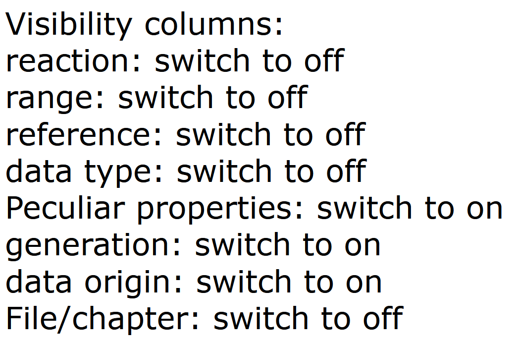
These columns except number are retractable and the user can freely choose the features to be shown through the Visibility column list at the top of the page: by clicking on/off a hidden/visible column is made visibile/hidden.
|
|
There are three additional columns that do not refer to data features but they contain some buttons to select the list of reaction data to be sent to the plotter or to the solver:
- not included in solver: one button for each group to remove any group element from the list of reaction to be sent to the solver,
- selected data: one button for each data to select one element of each group (radio button for group elements) to include in the list of reaction data to be sent to the solver - the header contains the clickable string unselect all to clear the list,
- plot: one or more buttons for each reaction data to be sent to the plotter - the header contains the clickable string unselect all to clear the list.
These buttons allows to send to the solver at most one element for each group of reaction data, while no restriction is made on the reaction data for the plotter.
On top of the first main table one can also find the alternative clickable strings show only selected reactions (rows)/show all reactions (rows) to show only those selected records for solver/all records. Similarly, the clickable strings show only selected reactions (Groups)/show all reactions (Groups) provides the same utility for all the elements of those groups containing the selected reactions.
III. PLOTTER
The reaction data selected through the third column (plot) are sent to the plotter that provides the plots with cross-sections/reaction rates on y-axis and energy/temperature on the x-axis. If the selected reaction data are cross sections PLOUTOS computes internally the reaction rate and plots it. Similarly, from interaction potentials both the corrresponding cross-sections and reaction rates are computed and plotted.
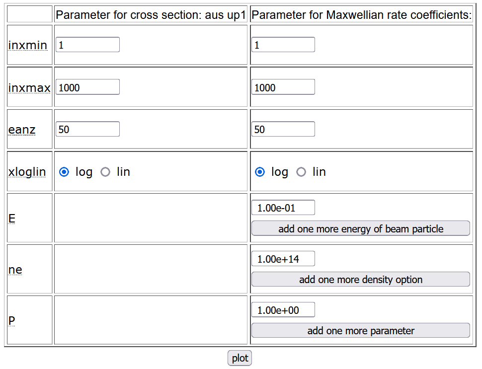
At the bottom of PLOUTOS initial page one can find to the right the table to set the plotter options.
|
It contains two columns: one for cross-section and one for reaction rate plots. The first two rows define the minimum and maximum values in eV for energy and temperature. The third row fixies the number of points, while the fourth one contains radio buttons to set the scale for the x-axis, whether logarithmic (log) or linear (lin). The last three rows are for reaction rates only and they can be used to fix additional parameters:
- energy for data in chapters H.3 and H.9,
- density for data in H.4 and H.10,
- other additional parameters.
|
|
For each additional parameter more values can be assigned by clicking on the buttons below the entries.
Below the table one can find the button plot to access the plotter.
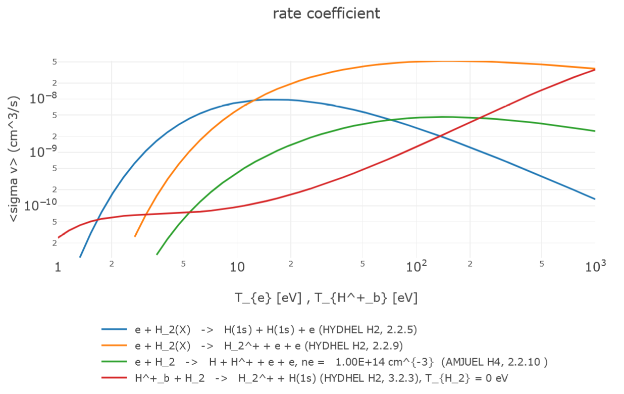
The *plotter page shows the graphs for the selected cross sections (for H.0 or H.1 data) as a function of center-of-mass energy and for the reaction rates as a function of beam temperature (see the figure below). At the top of the page one can download input and output data in various formats (db, fhg and json). The plots can be customized by showing/hiding the legend, by setting logarithmic scales on X and/or Y axis and by changing X and/or Y ranges, clicking the button re-draw button to apply the changes. Other graphical options (such as zoom, download as png, reset axis) are available by moving the cursor on the plot at the top right.
IV. SOLVER
The solver allows the user to solve a 1-dimensional linear collisional-radiative model (CRM) defined by the list of selected reaction data through the column selected data in the main tables of the initial page. Data for cooling rate (corresponding to chapters H.8, H.9, H.10) and for elastic reactions cannot be selected since they are irrelevant: the former are for energy distribution and the latter refer to processes that do not change particle concentration.
It is possible to save such a list in json format through the button save configuration at the botton of the page and to load a previously saved list by loading the corresponding json file through the button Start with own configuration at the top of the page.
The 1-dimensional characted of the CRM can be interpreted as time evolution or as space distribution. This features allow to model a finite velocity for each species and to perform a spectral analysis outlining the relevant time/spatial scales.
|
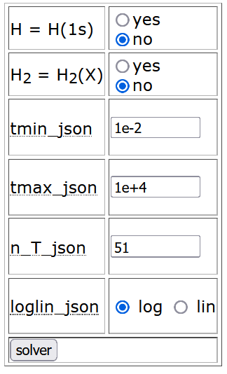
Some solver options can be fixed thorugh the table at the botton of PLOUTOS initial page to the left. It contains two rows to identify (yes) or treat as different (no) atomic (H) or molecular (H2) species with respect to their electronic ground state H(1s) and H2(X), respectively (this is a resonable assumption in most cases). The next four rows fix some options for the time variable: the minimum and maximum time, the number of points and the scale, whether logarithmic (log) or linear (lin) one.
By clicking the solver button, one enters the species selection page in which different options for the reactants and the products of the selected reaction data can be chosen.
|
|
The first table in the species selection page contains all the reactants and products as records whose feature columns are:
- select: to select the species to include into the solver, with the buttons to select/unselect all the listed species in header,
- species: with species name, derived from the databases,
- initial condition/incident flux: to fix the initial condition, i.e. the concentration at initial time t=0 (time evolution) or the incident flux at x=0 (spatial distribution),
- influx: to fix the external source influx,
- velocity,
- loss time,
- P, Q: to select whether the corresponding species is P, i.e. it is tracked normally, or it is a short-living Q species (according to Greenland classification ref.),
- sensitivity,
- most probable paths,
- plot/print: to select the species to be shown in output (plot or file), with the buttons to select/unselect all the listed species in header,
- reservoir: to select additional reservoirs having fixed temperature and density, default reservoirs being electrons, photons and bulk ions only.
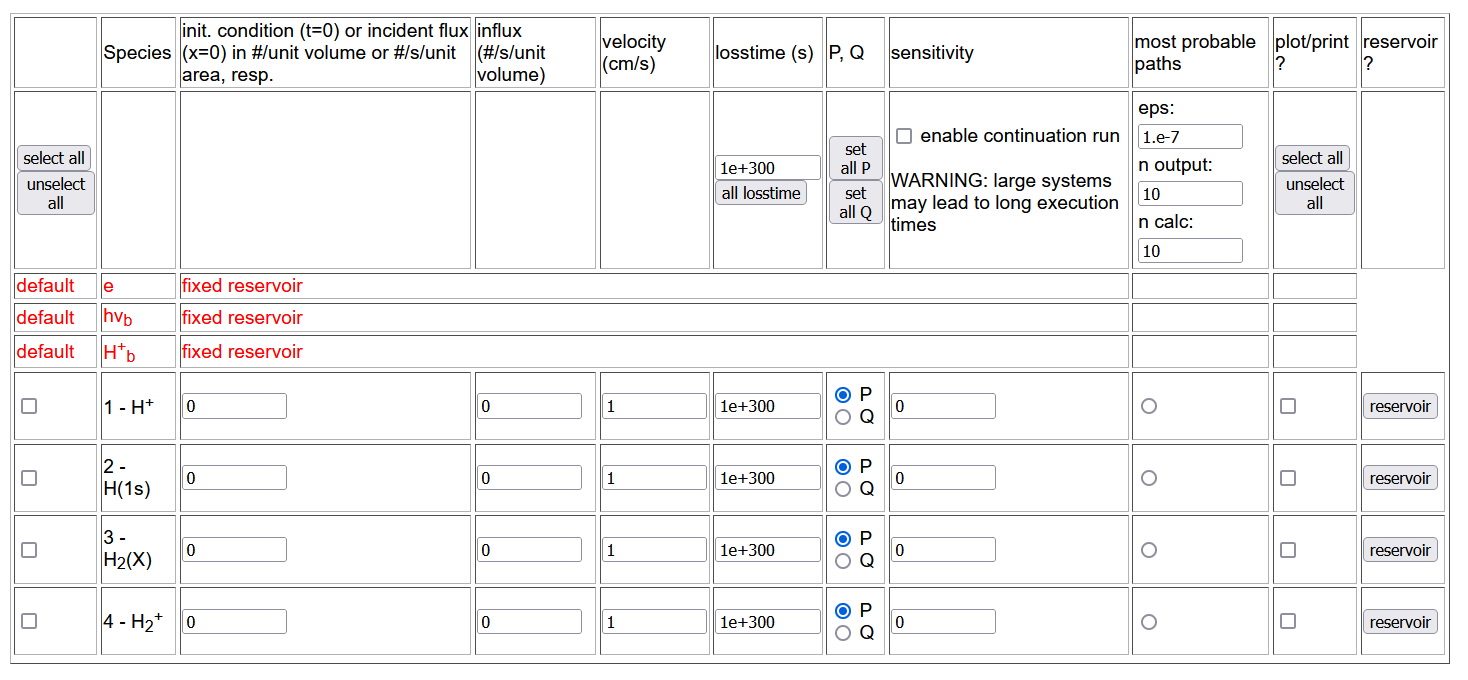
Additional tables allow the user to select the temperature and density of the reservoirs (in red), the maximal time, the thereshold value below which the rate is assumed to vanish (for ill-conditioned CRMs), the output (linear or logarithmic) scale for x (time/space coordinates) and y (concentration) axis.
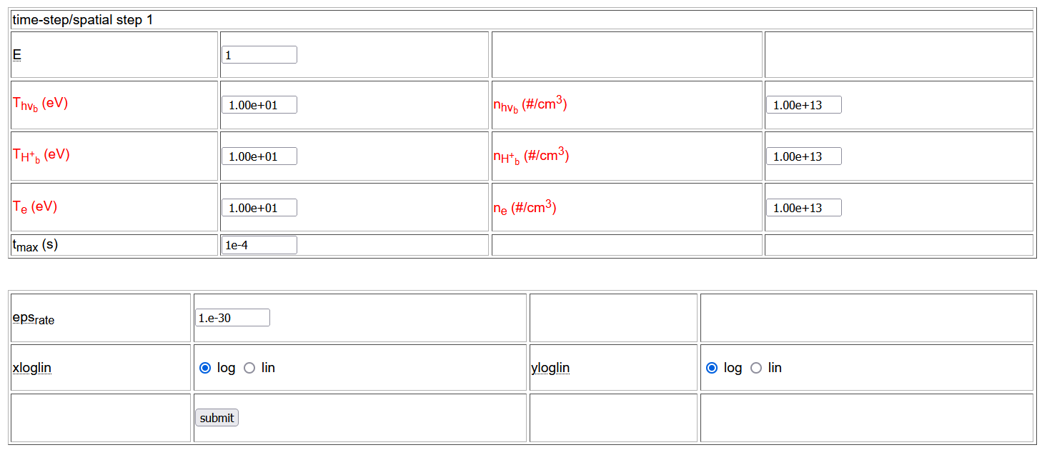
After setting the options the user can send the corresponding CRM to the solver and inspect the output through the submit button at the bottom of the species selection page .
|
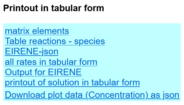
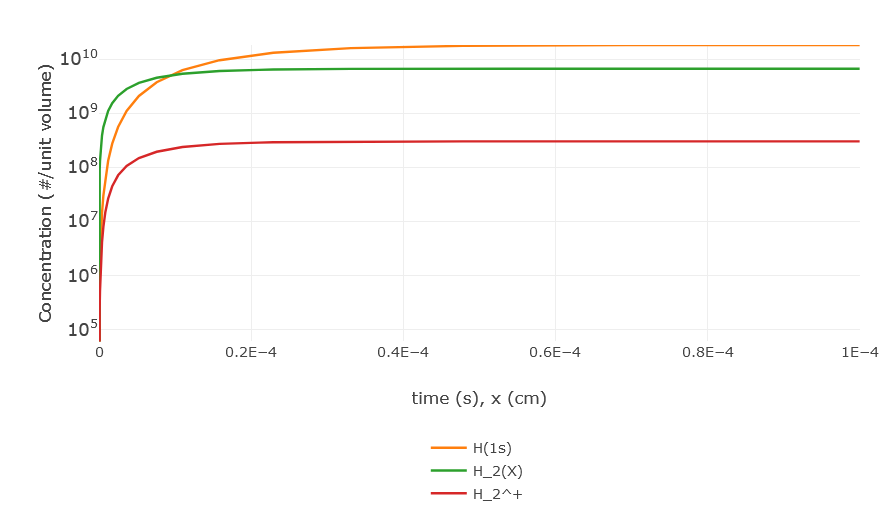
The solver output page provides several tables and plots outlining the results of the CRM. A first table presents a resume of the selections done in previous page (species, influx, ..), while the output files can be downloaded by clicking the printout list (see the image to the right). Then, one can find the plot of the species concentrations vs time/spatial coordinate (see the figure below), that is customizable as in the plotter page, and a technical summary of the solver run is presented.
|
|
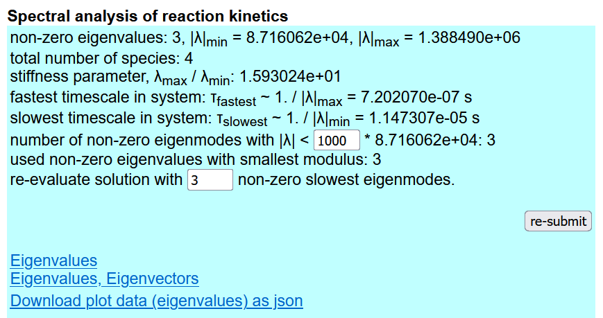
Next, the user can find the results of spectral analysis (see the figure below). The thresehold eigenvalue absolute value |λ| and the maximal number of non-vanishing eigenvalues can be changed with respect to the shown values and the analysis can be redone clicking the re-submit button. The last lines contains the clickable links for downloading the results. Finally one finds the plot of the minimal non-vanishing eigenvalue absolute value with respect to the eigenvalue number up to the maximal one.
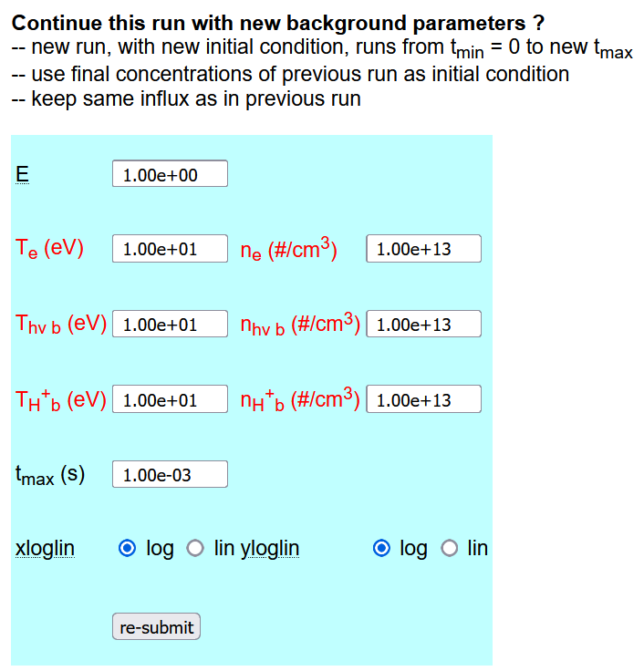
The bottom part of the solver output page allows the user to change some of the background parameters and peform a new run on top of the old one (i.e. the final concentrations are taken as initial conditions) by clicking the re-submit button.
V. Default cases
|
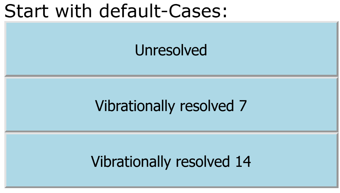
H2-F.Cianfrani,2022-2023: Default cases for molecular hydrogen decay can be selected through the buttons placed at the top of the initial page. They correspond to the vibrationally unresolved case and to the two vibrationally resolved cases, with 7 and 14 internal states, whose reaction data are shown in the table below (in the last column vibr.res. specify the source for the vibrationally-resolved cases if different from that in the unresolved one).
|
|
| Formula |
Type of reaction |
Source (database,chapter,number) |
| H2 + e → H2+ + e + e |
molecular ionization |
HYDHEL H.2 2.2.9,
H2VIBR H.2 2.[ν]vl4 vibr.res.
|
|
H2 + e → H2(btriplet) → H + H + e
|
neutral dissociation |
HYDHEL H.2 2.2.5,
H2VIBR H.2 2.[ν]vl1 vibr.res.
|
|
H2 + e → H + H+ + e + e |
dissociative ionization |
AMJUEL H.4 2.2.10 |
|
H2 + H+ → H2+ + H |
charge exchange |
HYDHEL H.2 3.2.3,
H2VIBR H.2 2.[ν]vl2 vibr.res.
|
|
H2(ν) + e → H2(ν ± 1) + e |
ladder-like vibrational transitions |
H2VIBR H.2 2.[ν]v[ν ± 1] vibr.res.
|
|
H + e → H+ + e + e |
ionization |
AMJUEL H.4 2.1.5 |
|
H2+ + e → H + H+ + e |
neutral dissociation (MAD) |
AMJUEL H.4 2.2.12 |
|
H2+ + e → H+ + H+ + e + e |
dissociative ionization (MAI) |
AMJUEL H.4 2.2.11 |
|
H2+ + e → H + H |
dissociative recombination (MAR) |
AMJUEL H.4 2.2.14 |
In the unresolved case one needs to identify H2 with H2(X) and the resulting CRM is non-trivial only if a non-vanishing H2 influx is chosen in the species selection page. In the two vibrationally resolved cases the user can freely split the full molecular source over different states H2(ν).
|